
How a single photon can induce 100-photon-worth of radiation pressure
Published:
I have recently got a chance to read this seminal paper by Yakir Aharonov et al., where a major surprise of the work is that, for a certain construction of the spin measurement of spin-1/2 particles, the apparent readout of the spin of a single particle can be arbitrarily larger than 1/2 (e.g., 100). While their main results are provided in a generic language, the thought experiment considered in the paper is a somewhat involved Stern-Gerlach experiment using electrons, which I struggled to digest as a one from nonlinear optics. The aim of this post is to show a simple nonlinear-optical reformulation of their thought experiment, hopefully providing useful intuitions to those with quantum and/or nonlinear optics background. Specifically, we construct a concrete example where single-photon can induce 100-photon-worth of radiation pressure.
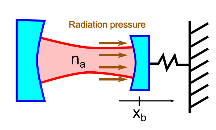
For the following, let us consider an optical cavity with a moving mirror on a spring. Inside the cavity, the position degree of freedom of the mirror is coupled to the photon mode via radiation pressure. The Hamiltonian of the system takes a well-known pondermotive form
\[H=-ga^\dagger ax_b\label{eq:hamiltonian}\]with \(g>0\), where \(a\) is the annihilation operator for the photon mode, and \(x_b=(b+b^\dagger)/2\) is the position operator for the moving mirror. Here, \(b\) is the annihilation operator for the mechanical excitation of the mirror. In our recent work, we also show an all-optical means to realize \eqref{eq:hamiltonian} using an optical parametric amplifier.
For concreteness, we consider the initial system state of the form \(\vert\varphi_\mathrm{i}\rangle_a\vert 0\rangle_b\), where \(\vert\varphi_\mathrm{i}\rangle_a=\sum_{n=0}^{n_\mathrm{max}}c_n\vert n\rangle_a\) is the photon-number state representation of the initial photonic state, and \(\vert 0\rangle_b\) is the vacuum state for the mechanical mode. For this initial state, we can analitically solve for the following system dynamics as
\[\vert \psi(t)\rangle=e^{-\mathrm{i}Ht}\vert\varphi_\mathrm{i}\rangle_a\vert 0\rangle_b=\sum_{n=1}^{n_\mathrm{max}}c_n\vert n\rangle_a\vert \beta_n\rangle_b\]where \(\vert \beta_n\rangle_b\) is a coherent state with $p$-displacement \(\beta_n=\mathrm{i}gtn\). Notice that the form of \(\vert \psi(t)\rangle\) implies that the momentum of the moving mirror increases by an amount proportional to the number of photons in the cavity.
Here, based on this setup, let us consider a somewhat trivially sounding question: “For a given maximum photon number \(n_\mathrm{max}\), what is the maximum amount of momentum that the moving mirror can gain from the radiation pressure?”
Because there can never be more than \(n_\mathrm{max}\) photons in the cavity, this should provide an upper bound to the achievable radiation pressure, and therefore, the answer should be $gtn_\mathrm{max}$. This can also be confirmed analytically via
\[\mathrm{argmax}_{\{c_n\}}\langle \psi(t)\vert p_b\vert\psi(t)\rangle=n_\mathrm{max}gt,\]where \(p_b=(b-b^\dagger)/2i\) is the momentum operator for the moving mirror.
Then, what if we allow postselections based on the final state of the light? More formally, conditioned on that the finial photon state in is found in a target state \(\vert\varphi_\mathrm{f}\rangle_a\), the post-selected mechanical state becomes
\[\vert\varphi'\rangle_b\propto{}_a\langle \varphi_\mathrm{f}\vert\psi(t)\rangle\]up to a normalization. Can the upper bound for the average momentum increment change for this post-selected state?
A common sense tells us that the answer should be “No”, because no matter how we “cherry pick” the measurement results based on the final photon state, we should never be able to find a case where there are more than \(n_\text{max}\) photons in the cavity. Therefore, the maximum momentum increment should be achieved when we find \(n_\mathrm{max}\) photons in the cavity at the point of measurement (i.e., \(\vert\varphi_\mathrm{f}\rangle_a=\vert n_\text{max}\rangle_a\)), leading to the same result \(\langle \varphi'\vert p_b\vert\varphi\rangle_b=n_\mathrm{max}gt\).
However, to our (at least my) surprise, it turns out that specially designed post-selection condition \(\vert\varphi_\mathrm{f}\rangle_a\) can break this bound, resulting in an arbitrarily large amount of momentum increment of the mirror. To see this concisely, we assume \(n_\text{max}=1\) and
\[\vert\varphi_\mathrm{i}\rangle_a=\frac{1}{\sqrt{2}}(-\vert 0\rangle_a+\vert 1\rangle_a).\]For the final photon state, we choose
\[\vert\varphi_\mathrm{f}\rangle_a=\frac{1}{\sqrt{2}}(\sqrt{1-\epsilon}\vert 0\rangle_a+\sqrt{1+\epsilon}\vert 1\rangle_a)\]with $0< \epsilon\ll 1$, leading to
\[\vert\varphi'\rangle_b\propto-\sqrt{1-\epsilon}\vert 0\rangle_b+\sqrt{1+\epsilon} \vert igt\rangle_b \label{eq:sum}.\]Specifically, when \(gt\ll 1\) holds true, we can approximately write
\[\vert\varphi'\rangle_b\sim -\sqrt{1-\epsilon} \vert 0\rangle_b+\sqrt{1+\epsilon} (\vert 0\rangle_b+igt\vert 1\rangle_b)\] \[\quad\quad=(\sqrt{1+\epsilon}-\sqrt{1-\epsilon})\vert 0\rangle_b+igt \sqrt{1+\epsilon}\vert 1\rangle_b\] \[\quad\quad\sim\epsilon\vert 0\rangle_b+igt \vert 1\rangle_b.\]For this post-selected state, the average momentum shift is
\[\langle\varphi'\vert p_b\vert \varphi'\rangle_b=n_\text{eff}gt\]with \(n_\text{eff}=\frac{\epsilon}{\epsilon^2+(gt)^2}\), which can be seen as \(n_\text{eff}\)-photon-worth of average momentum shift. Notably, \(n_\text{eff}\) is not necessarily upper bounded by \(n_\text{max}=1\), and in fact, \(n_\text{eff}\) can be arbitrarily large. To see this concretely, we can consider \(gt=\epsilon\), where we find \(n_\text{eff}=\epsilon^{-1}/2\), which can be made arbitrarily large in the limit of \(\epsilon\rightarrow 0\).
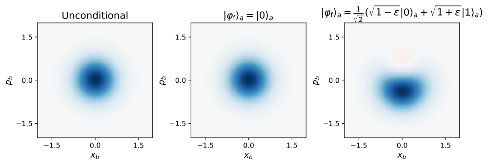
The figure attached shows a numerical demonstration using QuantumOptics.jl; Both the unconditional state \(\vert\psi(t)\rangle\) and the naively chosen post-selected state \(\vert\varphi_\mathrm{f}\rangle_a=\vert1\rangle_a\) exhibit momentum increment below the bound $gt$. However, for the specifically designed post-selecting condition with \(gt=\epsilon\), the post-selected state becomes an equal superposition of 0 and 1 photon state \(\vert\varphi'\rangle_b=\frac{1}{\sqrt{2}}(\vert0\rangle_b+i\vert1\rangle_b)\), which exhibits a constant momentum increment of \(\langle\varphi'\vert p_b\vert \varphi'\rangle_b=1/2\), no matter how small \(gt\) is. For the parameters used here (\(gt=\epsilon=1/200\)), this amount of momentum increment corresponds to \(100\)-photon-worth of radiation pressure.
So what is the cause of such a counter-intuitive outcome? In the following, we argue that this stems from the implicit “classical intuitions” that we assume when adding Gaussian probability distributions.
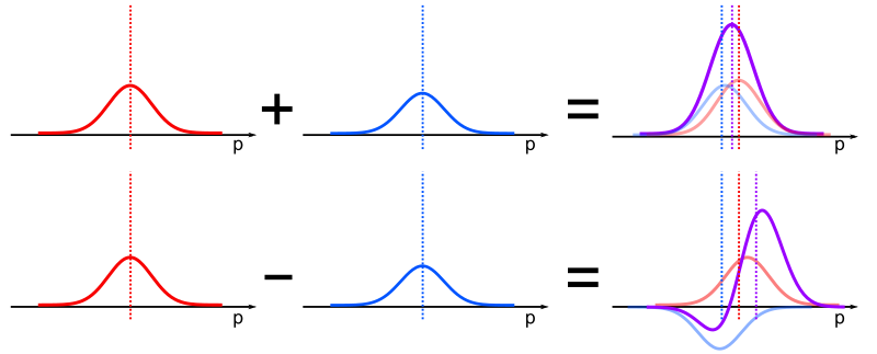
Assume we add two Gaussian wavefunctions in the momentum space with the same variance $\sigma$ and amplitude; one at the origin $p=0$ and the other one around $p=d$. When the variance is much larger than the separation (i.e., $\sigma\gg d$), the centroid of the overall distribution is trivially given as the average of centroids of the two distributions, i.e., \(\langle p\rangle=d/2\). Even if we allow the relative amplitude between two wavefunctions to change, it is obvious that the average centroid should be somewhere in between $p=0$ and $p=d$. We can interpret this as a classical (i.e., incoherent) way of adding probability distributions, which we argue is forming our “classical intuitions”.
However, in quantum mechanics, probability distribution is directly tied to wavefunctions with complex phases, which can make a critical difference from the classical scenario via interference effects; When two Gaussian wavefunctions with the same variance and similar amplitude are added with opposite sign, the resultant distribution shows a vastly skewed and non-Gaussian form due to the interferences. And as depicted in the figure attached, this skewness of the resultant probability distribution can actually push the centroid beyond the interval of \([0,d]\). Notice that \eqref{eq:sum} is exactly reproducing this situation of two Gaussian wavefunctions being added with opposite signs, where she signs are introduced by the specific choice of \(\vert\psi_f\rangle_a\).